It’s easy to see what content gets traffic. It’s one of the most popular reports in Analytics. The All Pages report is sorted by pageviews so it’s all right there. Most marketers know their top traffic pages.
It’s hard to see what content gets conversions. There isn’t a report in Google Analytics that shows the conversion rates of your articles. That’s why very few marketers know their top converting pages.
Of all the articles you’ve published, which ones inspire visitors to subscribe to your newsletter? Which grow your list? Some are much better at this than others.
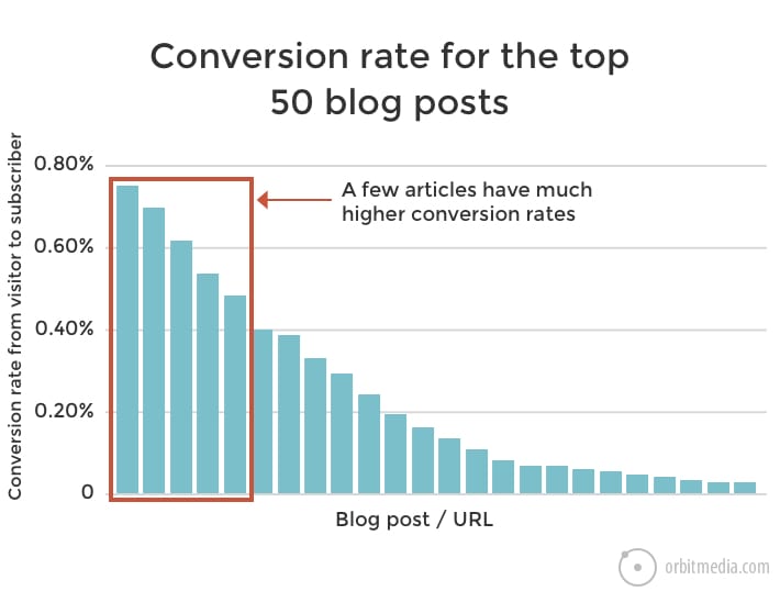
Your top converting articles are far more compelling than the rest. The conversion rate on the top 10 is probably 10x the average. They are your very best articles, according to your audience.
To find these champs, you’ll pull data from two reports:
- Reverse Goal Path: This report shows the pages that visitors were on just before they converted and the total number of conversions for each.
- All Pages: This report shows the number of views on those pages.
So we have the total conversions in one report and the unique pageviews in another. If we divide the first number by the second, we’ll have the conversion rate. We’ll do all it using Google Analytics and Google Sheets. And through the magic of scheduled reports, we can do it once and it will stay up-to-date forever.
Connecting Google Analytics and Google Sheets
We’ll start from the very beginning. But this process assumes that you already have your Google Analytics Goals set up!
1. Get the Google Analytics add-on
Open a new Google Sheet and click on “Add-ons” in the menu. One of the items in the dropdown is “Get add-ons.” Click it and you’ll see a gallery of add-ons with Google Analytics at the top. Add it!
2. Create a new report for “Conversions”
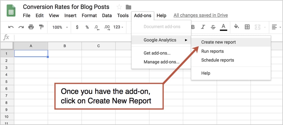
Now that the add-on is in place, that same menu will show the GA add-on and a new submenu. Select “Create new report.”
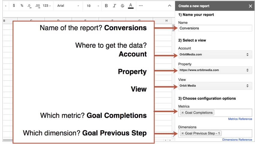
For the first report, we’ll get the total conversions for each page, just as if we were looking at the Reverse Goal Path report. Name the report “Conversions” (a one-word name is best) and select your Google Analytics Account, Property and View.
Finally, we’ll choose the configuration options.
- Metric: Goal Completion
- Dimension: Goal Previous Step – 1
Note: this assumes the visitor can subscribe directly on the article page and subscribers land on a thank you page. So the article is previous step one in that process. But this isn’t always the case. Here are two scenarios:
- On your site, if the visitor has to go from the article to a separate page to subscribe, then set the dimension as “Goal Previous Step – 2”
- On your site, if the visitor can subscribe without going to a thank you page (maybe you have an opt-in pop-up window with a thank you message and no thank you page) then set the dimension as “Goal Completion Location”
It should look like this:
Click the blue “Create Report” button at the bottom. Once complete, Sheets will have a new tab called “Report Configuration.” We’ll come back to that in a minute.
3. Create a new report for “Pageviews”
Using the same process, we’ll import data for the second report we’ll need. We’ll name it “Pageviews” and use the same account, of course. Here are the configuration options:
- Metric: Unique Pageviews
- Dimension: Page
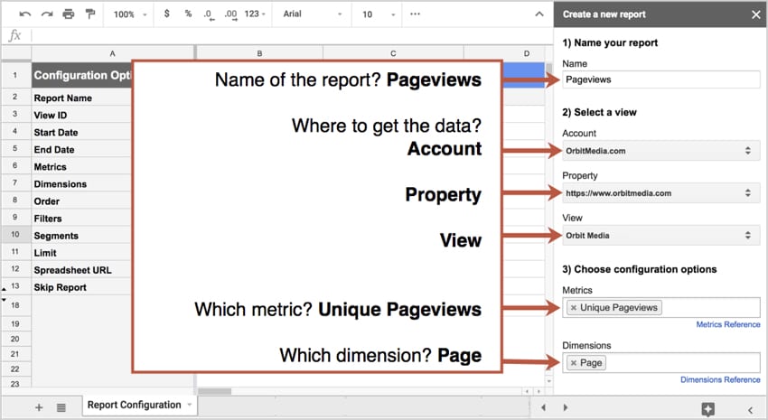
Click the “Create Report” button and Sheets will add a new column to the “Report Configuration” tab. It should look like this:
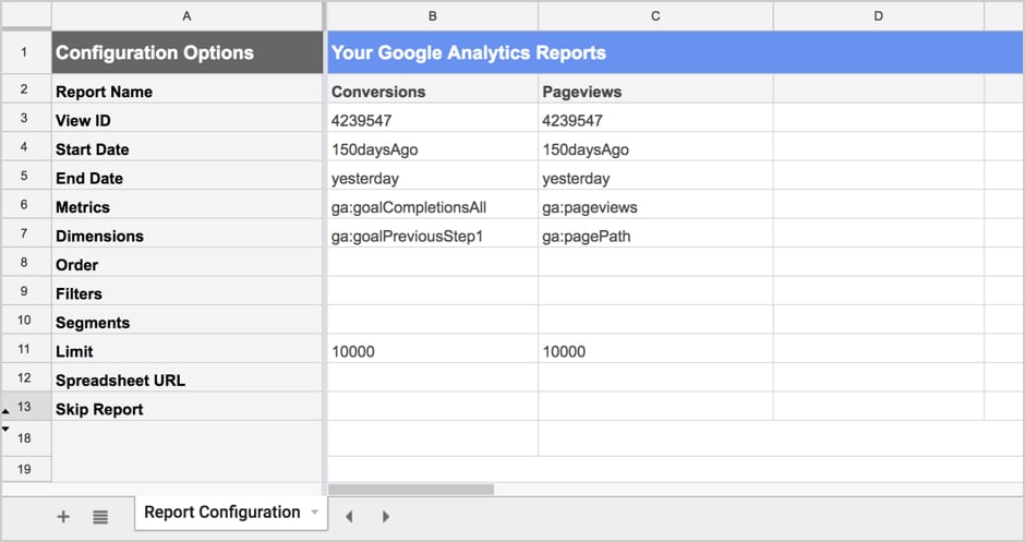
In this screenshot, you can see I’ve adjusted the Start Date and Limit, to get more data. If at the end of step eight you don’t have much data, you may want to do the same.
4. Run the reports
Next, we’ll run the reports. From the Add-ons menu, select Google Analytics > Run Reports. Now Google Sheets imports the data from Google Analytics and makes a new tab for each report.
Once the data is in the spreadsheet, all of you Excel experts are free to run wild and start doing calculations. But for anyone who needs a bit more spreadsheet help (like me) here are the steps to get that conversion rate calculated…
Combing the data into a single report
It’s easiest to calculate if we can first get all the data into the same tab.
5. Start a new tab for the final report
This one we’ll call “Conversion Rate Per Blog Post” since that’s what we’re going to calculate.
6. Pull in the data
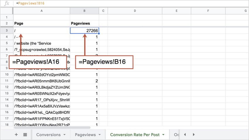
First, we’ll bring in the data from the “Pageviews” tab. We’ll have two columns, one for the page and one for the unique pageviews.
Here are the names of the columns and the values to enter in the cells below:
Column A:
- Cell A2 name “Page”
- Cell A3 enter “=Pageviews!A16“
Column B:
- Cell B2 name “Pageviews”
- Cell B3 enter “=Pageviews!B16“
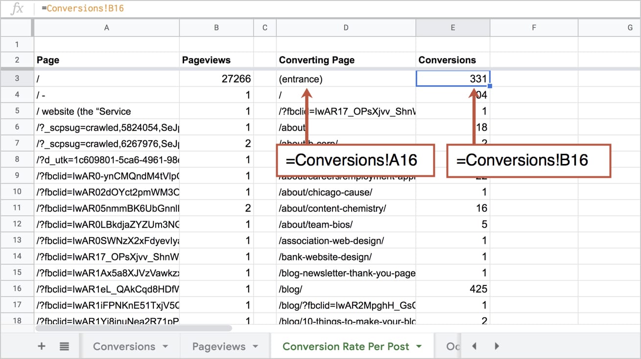
This should pull in all the pages and pageviews from the other tab. Next, we’ll do it for the next two columns, bringing in data from the conversions report.
Column C: Leave blank as a spacer
Column D:
- D2 name “Converting Page”
- D3 enter “=Conversions!A16“
Column E:
- E2 name “Conversions”
- E3 enter “=Conversions!B16“
Now we have all the data we need in one place! But it’s still not ready for the calculation.
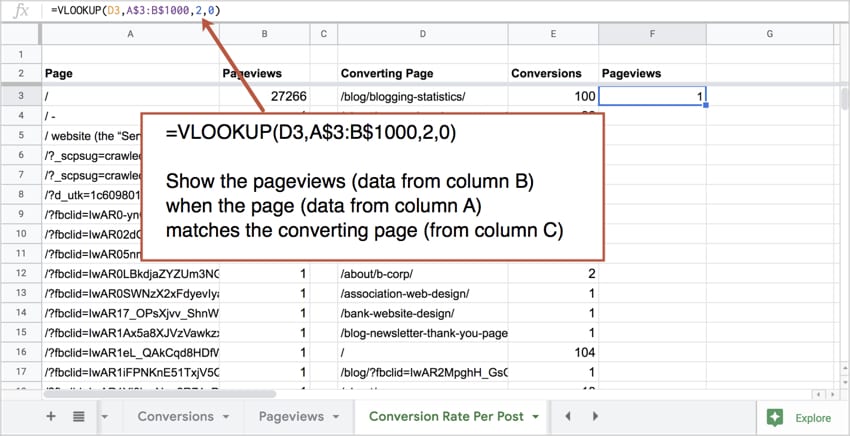
7. Match the pages using a VLOOKUP
Right now, our pages are listed here in two rows. We need to match them up so we can show Pageviews in a new column. This is what the VLOOKUP function is for.
Without getting into the details of the parameters, here is what the values should look like based on everything we’ve done so far.
Column F:
- Cell F2 name “Pageviews”
- Cell F3 enter “=VLOOKUP(D3, A$3:B$1000,2,0)“
This tells Sheets to take everything from column D (converting pages) and look for exact matches in column A (pages), and when it finds them, to put the data from column B (pageviews) into column F. Make sense?
I’ll be honest, I got help from my wife on this. Thanks, Crystal!
You’re almost finished. All the data is in the right places. One last step…
8. Calculate the conversion rate!
Now the easy part. For the seventh and final column, tell Sheets to divide the Conversions (column E) by the Pageviews (column F). Calculating the conversion rate.
Column G:
- Cell G2 name “Conversion Rate”
- Cell G3 enter “=E3/F3“
Actually, the conversion rate is the percentage of visits (not visitors) that included a goal completion. It is a sessionized metric, based on visits, not visitors. That’s why we’re using unique pageviews, which is the number of visits in which that page was viewed.
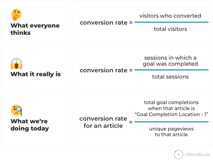
Another time, we can talk about conversion rate misconceptions and the common Analytics settings that make them inaccurate and/or meaningless.
Here’s what your report will look like.
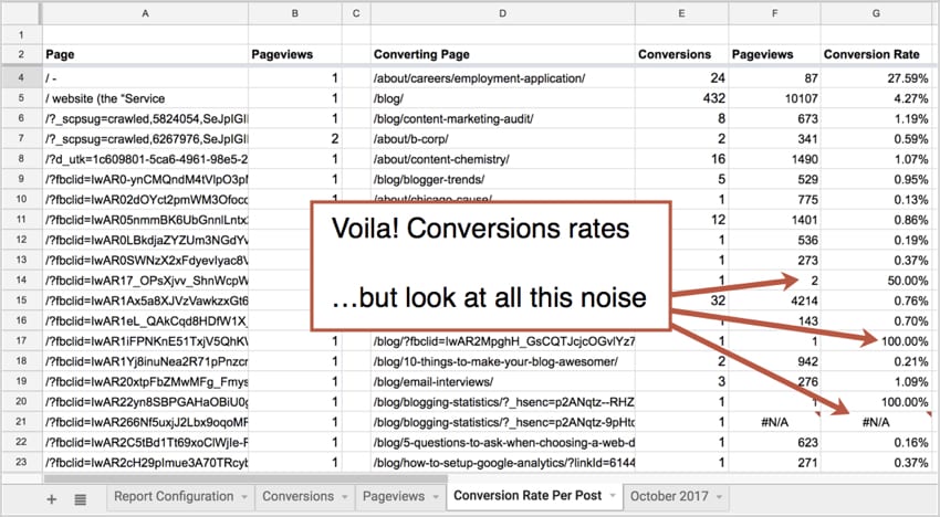
We are very close! But there is still a lot of noise in the report. Outliers, useless data and #N/A values. It’s clean up time…
9. Clean up, sort and filter
Again, if you’ve got the spreadsheet skills, you know what to do. For the rest of us, here are some tips for filtering and sorting.
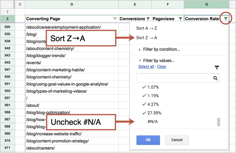
Click on any cell in the conversion rate column, then click the Funnel icon in the menu to turn on filters.
- Conversion Rate column: Sort Z to A (so the cream rises to the top!)
- Conversion Rate column: Filter out #N/As (this takes out the rows where the pages didn’t match)
- Conversions Column: Filter by condition, greater than 3 conversions (if there weren’t at least a few, the data isn’t meaningful)
10. Analyze
Here it is. A list of your best stuff according to your visitors. These are the pages that inspire action and grow your list. If you like charts, make one!
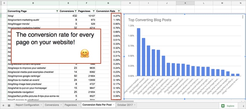
Notice how much more compelling some posts are than others. The top post likely has 10x the conversion rate than the post at the bottom of the list. And most of your content converts so few visitors that it doesn’t appear on the list at all.
Now you know exactly what to prioritize, to promote, to push hard.
Bonus! Update this report automatically forever
As a final step, you can run the reports behind this data on a regular schedule. It’s easy.
From the menu, go to Add-ons > Google Analytics > Schedule reports. Check the box to “Enable reports to run automatically.” Then choose the interval: monthly, weekly, daily or hourly.
Last screenshot. I promise!
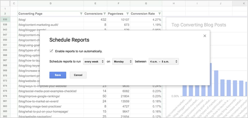
I have mine run on Monday mornings at 5am. I’ll have conversions rates with my coffee.
Now put on your traffic driving gloves
The Orbit blog is filled with posts about driving traffic. But here are 10 to get you started.
Remember, visits to these posts are 10x to 100x more effective than your average article. In other words, one visit to these is worth 100 visits to your average post.
- Put these posts into heavy social rotation
- Feature these on your homepage
- Feature these at the top of your blog
- Link to these posts from your top traffic posts
- Link to one of these from your email signature
- Syndicate these on LinkedIn and Medium
- Write a related guest post that links to one of these
- Promote these with social media videos
- Create a welcome series email that links to these
- Link to one from your contact form’s thank you page
And of course, now that you know your greatest hits, you know what topics to focus on. Consider aligning your content strategy with these. Drop the topics that don’t appear and double down on the topics that do.